
Causal Impact: state-space models in settings where a randomized experiment is unavailable
TL;DR: There are ways of measuring the causal impact of some business intervention even in scenarios where a randomized experiment is unavailable. In this post we investigated the increase in Google trends popularity index of some search terms caused by different interventions. The same logic can be applied in business contexts such as the impact of a new product launch, the onset of an advertising campaign and other problems in economics, epidemiology, biology among others.
Jupyter notebook with the code for this post
Motivation
At work, you are responsible for making many decisions that can impact aspects of your business in different ways. Most of the time, there are simple approaches to measure the impact of these decisions.
You launched an advertising campaign and, looking at sales that increased by 5% a month later, concluded that your campaign was a success. Right? Well, did you do a random experiment? Did you consider other factors such as seasonality or sales trend?
Similar to this scenario, there are a plethora of other cases in which we may be interested in measuring the causal impact of the action.
Causal Impact by Google
There are some complex aspects of infering the causality of an intervention. In 2015 some awesome researchers from Google, published a paper entitled: “INFERRING CAUSAL IMPACT USING BAYESIAN STRUCTURAL TIME-SERIES MODELS”.
Along with the paper they also introduced CausalImpact, an R package (there is also a Python port by Dafiti) that implements their approach. In this tutorial we are going to use the Python version.
Quoting directly from the abstract of the paper:
This paper proposes to infer causal impact on the basis of a diffusion-regression state-space model that predicts the counterfactual market response in a synthetic control that would have occurred had no intervention taken place. In contrast to classical difference-in-differences schemes, state-space models make it possible to (i) infer the temporal evolution of attributable impact, (ii) incorporate empirical priors on the parameters in a fully Bayesian treatment, and (iii) flexibly accommodate multiple sources of variation, including local trends, seasonality and the time-varying influence of contemporaneous covariates
Measuring the causal impact of mentioning an unusual term on a popular brazilian TV show
Context
Big Brother Brasil (BBB) is an international TV show that is popular in Brazil and broadcast on prime time open television. One of the participants suggested, live, that another participant search Google for an unusual term that she had spoken. The unusual word was “sororidade” (“sorority”).
Many media outlets later reported that the episode caused searches for the term to increase 250%.
The episode took place on February 9, 2020 between 9 pm and 10 pm Brazilian time.
Let’s investigate the causality of the intervention in increasing interest in the term based on Google trends.
1. Gathering the data
We are going to download the data from Google Trends.
There are two main ways of doing this:
- We can navigate to the website and specify which term we are looking for, the region and timeframe
- We can do this directly in Python, using a third-party library such as pytrends
To install pytrends, switch to your preferred environment and run the command:
pip install pytrends
From the presentation of the causal impact, the author of the package suggests that we use between 5 and 10 related time series that can help to model the behavior of our time series of interest.
Therefore, we are going to download some common Brazilian terms in the same period that may help our Bayesian structural time series model to understand the search behavior of our target term.
from pytrends.request import TrendReq

pytrends = TrendReq(hl='pt-BR', tz=45)

kw_list = ["sororidade", "futebol", "carro", "temperatura", "restaurante"]
pytrends.build_payload(kw_list, cat=0, timeframe="2020-02-06T08 2020-02-13T07")

# the interest_over_time() method returns a pandas DataFrame
df = pytrends.interest_over_time()
| date | sororidade | futebol | carro | temperatura | restaurante | isPartial |
|---|---|---|---|---|---|---|
| 2020-02-06 08:00:00 | 0 | 1 | 2 | 9 | 4 | False |
| 2020-02-06 09:00:00 | 0 | 2 | 4 | 11 | 6 | False |
| 2020-02-06 10:00:00 | 0 | 2 | 7 | 13 | 8 | False |
| 2020-02-06 11:00:00 | 0 | 2 | 8 | 17 | 10 | False |
| 2020-02-06 12:00:00 | 0 | 2 | 10 | 22 | 13 | False |
2. Organizing the data
df = df.drop(columns=["isPartial"])

df.plot(figsize=[16,9])
sns.despine()
plt.ylabel("Interest over time (Google Trends)")
plt.xticks(rotation=45)
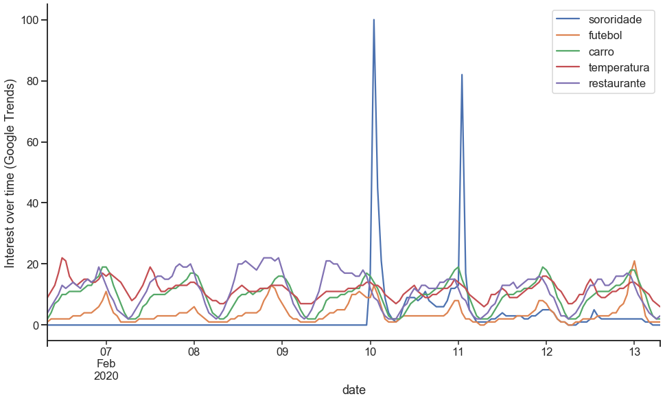
# changing the zeros to 0.1 so the model converge
df["sororidade"] = df["sororidade"].apply(lambda x: 0.1 if x==0 else x)
3. Causal Impact
pre_period = [
pd.to_datetime(np.min(df.index.values)),
pd.to_datetime(np.datetime64("2020-02-09T22:00:00.000000000")),
]
post_period = [
pd.to_datetime(np.datetime64("2020-02-09T23:00:00.000000000")),
pd.to_datetime(np.max(df.index.values)),
]
ci = CausalImpact(df, pre_period, post_period)
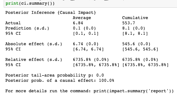
print(ci.summary())
Calling the summary method on the CausalImpact object we obtain a numerical summary of the analysis.
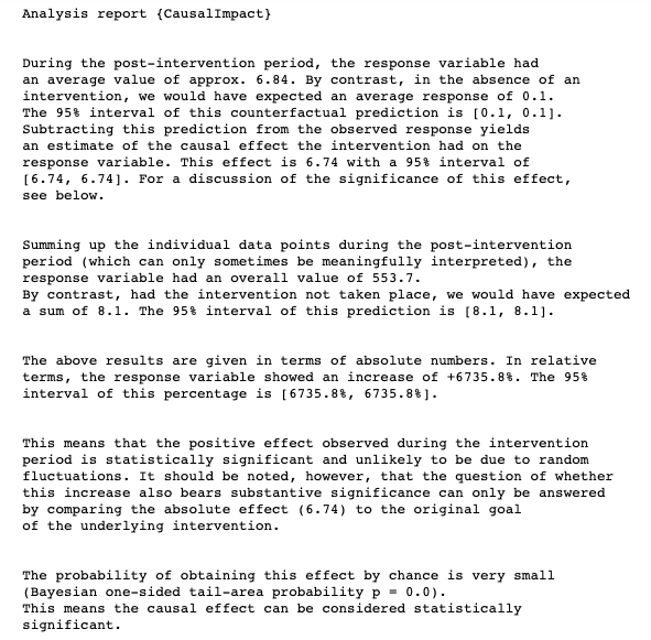
print(ci.summary(output='report'))
For additional guidance about the correct interpretation of the summary table, the package provides a verbal interpretation, printed using the same method but with output="report".
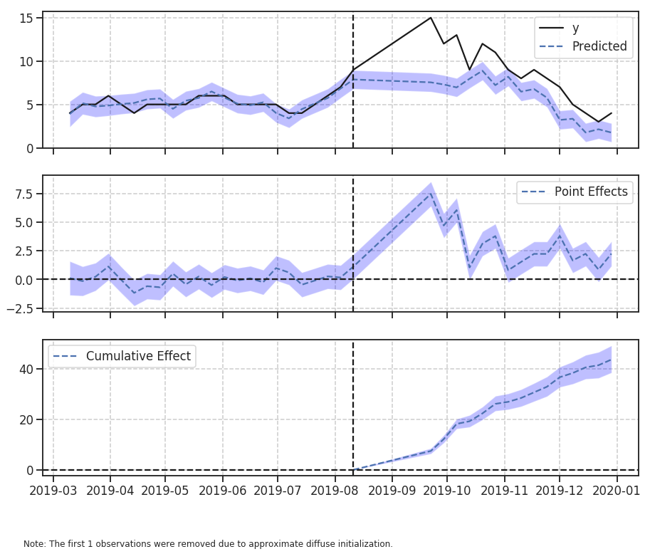
ci.plot()
Explaining the plots, in the package documentation:
“By default, the plot contains three panels. The first panel shows the data and a counterfactual prediction for the post-treatment period. The second panel shows the difference between observed data and counterfactual predictions. This is the pointwise causal effect, as estimated by the model. The third panel adds up the pointwise contributions from the second panel, resulting in a plot of the cumulative effect of the intervention.”
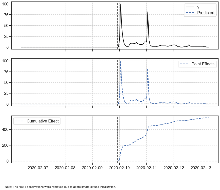
Just by looking at the sorority interest over time plot we may have concluded that it was obvious the causal effect.
In addition, the CausalImpact report is somewhat misleading: our series had a lot of zeros, as it is an unusual term and we have counted the metrics of interest from Google trends over time. Because of this, all changes are greatly expanded, and this reflects the increase of +6735.8% in the response variable.
Let’s look at another example to consolidate our understanding.
Another example - Amazon rainforest burns
Context
From wikipedia:
“The forest fires in the Amazon in 2019 were a series of forest fires that affected South America, mainly Brazil. At least 161.236 fires were recorded in the country from January to October 2019, 45% more compared to the same period in 2018, which reached 84% in August”
Also from the same article:
“On August 11, Amazonas declared a state of emergency. NASA images showed that on August 13, smoke from fires was visible from space […]”
We will set August 11, 2019 as the intervention period for our causality study.
Causal Impact
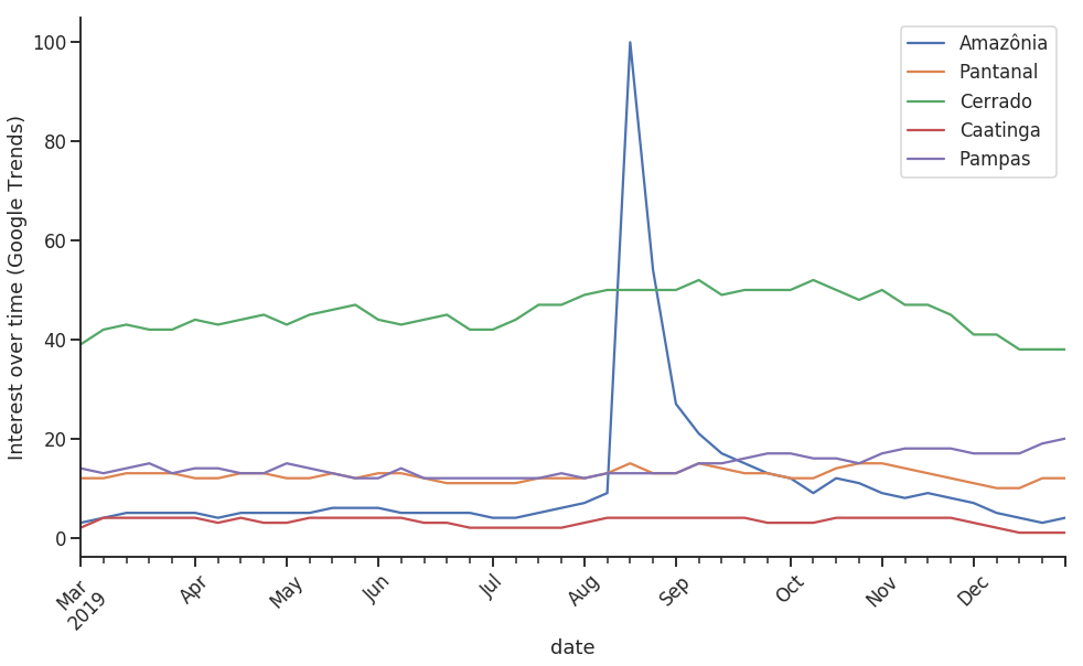
kw_list = ["Amazônia", "Pantanal", "Cerrado", "Caatinga", "Pampas"]
pytrends.build_payload(kw_list, cat=0, timeframe='2019-03-01 2020-01-01')

df = pytrends.interest_over_time()
| date | Amazônia | Pantanal | Cerrado | Caatinga | Pampas | isPartial |
|---|---|---|---|---|---|---|
| 2019-03-03 00:00:00 | 3 | 12 | 39 | 2 | 14 | False |
| 2019-03-10 00:00:00 | 4 | 12 | 42 | 4 | 13 | False |
| 2019-03-17 00:00:00 | 5 | 13 | 43 | 4 | 14 | False |
| 2019-03-24 00:00:00 | 5 | 13 | 42 | 4 | 15 | False |
| 2019-03-31 00:00:00 | 5 | 13 | 42 | 4 | 13 | False |
df = df.drop(columns=["isPartial"])
pre_period = [
pd.to_datetime(np.min(df.index.values)),
pd.to_datetime(np.datetime64("2019-08-11")),
]
post_period = [
pd.to_datetime(np.datetime64("2019-09-22")),
pd.to_datetime(np.max(df.index.values)),
]
ci = CausalImpact(df, pre_period, post_period)
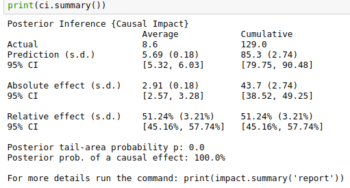
print(ci.summary())
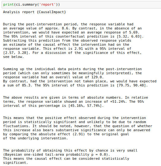
print(ci.summary(output='report'))
ci.plot()

Here we have something closer to what we find on a daily basis, but still a little exaggerated.
We see that the percentage increase in the response variable after the intervention was +51.24% and this change was statistically significant.
Final thoughts
The examples shown here help to illustrate the concept and API of the package.
I invite you to go further and try to create business scenarios in which this type of report can be useful. At work, I had no trouble finding these scenarios and it is your duty, as a data scientist, to provide data-driven value where you deem it appropriate.
References
- https://google.github.io/CausalImpact/CausalImpact.html
- https://github.com/dafiti/causalimpact
- https://www.uol.com.br/universa/noticias/redacao/2020/02/11/sororidade-buscas-no-google-crescem-250-apos-fala-de-manu-gavassi-no-bbb.htm
- https://www.huffpostbrasil.com/entry/sororidade-manu-gavassi_br_5e442423c5b61b84d3438b88
- https://emais.estadao.com.br/noticias/tv,bbb-20-buscas-por-sororidade-no-google-sobem-250-apos-fala-de-manu-gavassi,70003193892
- https://pt.wikipedia.org/wiki/Inc%C3%AAndios_florestais_na_Amaz%C3%B4nia_em_2019